Training a DQN Agent in Myriad

A complete Myriad training run: configure, train, analyse, and reproduce.

Three properties of Myriad training worth understanding up front:

Parallel by default. The training loop runs many environment instances simultaneously. Here we use 128 environments — more environments means more transitions per gradient step, stabilising learning without proportionally increasing wall-clock time.

Reproducible by design. Runs are deterministic given a seed on the same GPU hardware. The full config is saved alongside results — pass it back to train_and_evaluate() to get identical output. Minor numerical differences may occur across different GPU models or driver versions due to non-deterministic GPU kernel optimizations.

One unified API. The evaluate() call from Tutorial 01 works on trained agents too: pass the learned agent_state and get the same parallel rollout statistics.

We train on CartPole: balance a pole on a cart by pushing left or right. An episode ends when the pole falls past a threshold or the cart leaves the track. Max return is 500.

import matplotlib.pyplot as plt
from _helpers import setup_logging, side_by_side_videos

from myriad import (
    config_to_eval_config,
    create_config,
    create_eval_config,
    evaluate,
    load_run,
    train_and_evaluate,
)
from myriad.utils.plotting import plot_training_curve
from myriad.utils.rendering import render_episodes

setup_logging()

Section A: Baselines

Before training, we use the evaluate() API from Tutorial 01 to establish what non-learning controllers can achieve.

• Random: lower bound — acts without any knowledge of the state

• Bang-Bang: reacts to pole angular velocity, which prevents the pole from falling but ignores cart position — the cart gradually drifts off the track (~185/500)

DQN will need to learn both pole balance and cart position control to reach 500.

baselines = {
    "Random": dict(agent="random"),
    "Bang-Bang": dict(agent="bangbang", obs_field="theta_dot", setpoint=0.0),
}

baseline_results = {}
baseline_episodes = {}
for label, kwargs in baselines.items():
    config = create_eval_config(env="cartpole-control", eval_rollouts=50, seed=0, **kwargs)
    results = evaluate(config, return_episodes=True)
    baseline_results[label] = results
    baseline_episodes[label] = results.episodes
    print(f"{label}: {results}\n")

INFO:2026-02-23 16:45:31,210:jax._src.xla_bridge:822: Unable to initialize backend 'tpu': INTERNAL: Failed to open libtpu.so: libtpu.so: cannot open shared object file: No such file or directory
[16:45:31 INFO] Unable to initialize backend 'tpu': INTERNAL: Failed to open libtpu.so: libtpu.so: cannot open shared object file: No such file or directory
[16:45:32 INFO] Artifacts: outputs/2026-02-23/16-45-31
  ├── .hydra/  (config snapshot)
  ├── results.pkl  (metrics & config)
  └── run_metadata.yaml  (timing & status)

Random: EvaluationResults(
  mean_return=22.1 ± 10.9,
  range=[10.0, 57.0],
  mean_length=22.1,
  num_episodes=50
)

[16:45:32 INFO] Artifacts: outputs/2026-02-23/16-45-32
  ├── .hydra/  (config snapshot)
  ├── results.pkl  (metrics & config)
  └── run_metadata.yaml  (timing & status)

Bang-Bang: EvaluationResults(
  mean_return=184.5 ± 39.0,
  range=[131.0, 266.0],
  mean_length=184.5,
  num_episodes=50
)

Section B: Train DQN

create_config() + train_and_evaluate() is Myriad’s training API. The config captures everything: environment, agent, optimisation settings, and evaluation schedule.

128 parallel environments collect transitions simultaneously each step. A larger environment count means a larger, more diverse batch per gradient update — more signal, more stable training. With steps_per_env=5000, the total run is 640K transitions.

Key settings:

• num_envs=128 — parallel environments; directly controls batch diversity per update

• steps_per_env=5000 — training steps per environment (640K total transitions)

• eval_frequency=500 — evaluate every 500 steps/env, producing 10 checkpoints

• scan_chunk_size=500 — must match eval_frequency to avoid wasted computation

• epsilon_decay_fraction=0.4 — ε decays from 1.0 → 0.1 over the first 40% of training

• eval_episode_save_frequency=500 — save one episode per checkpoint for later rendering

config = create_config(
    env="cartpole-control",
    agent="dqn",
    num_envs=1,
    steps_per_env=50_000,
    eval_frequency=5_000,
    eval_rollouts=50,
    epsilon_decay_fraction=0.4,
    target_network_frequency=100,
    seed=0,
    # Enable episode saving
    eval_episode_save_frequency=5_000,
    eval_episode_save_count=1,
)
results = train_and_evaluate(config)
print(results)

# Get run directory for later use
run_dir = results.run_dir
print(f"\nRun saved to: {run_dir}")

[16:45:37 INFO] Step  5000/50000 ( 10%) | loss=6.291 | eval_return=179.54
[16:45:38 INFO] Step 10000/50000 ( 20%) | loss=33.734 | eval_return=183.98
[16:45:38 INFO] Step 15000/50000 ( 30%) | loss=15.617 | eval_return=151.58
[16:45:39 INFO] Step 20000/50000 ( 40%) | loss=10.461 | eval_return=209.32
[16:45:39 INFO] Step 25000/50000 ( 50%) | loss=1.181 | eval_return=130.58
[16:45:40 INFO] Step 30000/50000 ( 60%) | loss=1.776 | eval_return=500.00
[16:45:40 INFO] Step 35000/50000 ( 70%) | loss=8.480 | eval_return=500.00
[16:45:40 INFO] Step 40000/50000 ( 80%) | loss=3.172 | eval_return=472.60
[16:45:41 INFO] Step 45000/50000 ( 90%) | loss=1.983 | eval_return=500.00
[16:45:41 INFO] Step 50000/50000 (100%) | loss=1.157 | eval_return=500.00
[16:45:41 INFO] Artifacts: outputs/2026-02-23/16-45-32
  ├── .hydra/  (config snapshot)
  ├── episodes/  (10 step checkpoints)
  ├── results.pkl  (metrics & config)
  └── run_metadata.yaml  (timing & status)

TrainingResults(
  final_eval_return=500.0 ± 0.0,
  steps_per_env=50,000,
  global_steps=50,000,
  num_evals=10
)

Run saved to: outputs/2026-02-23/16-45-32

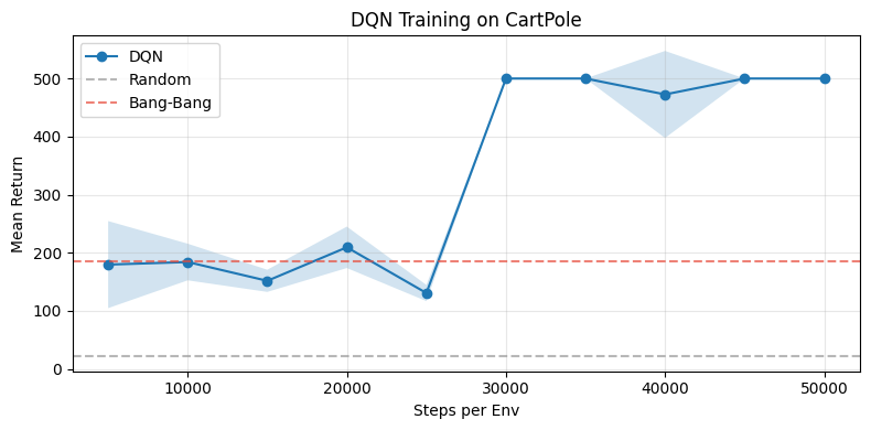
Section C: Learning Curve

DQN’s mean return at each evaluation checkpoint, with baseline scores as reference lines.

DQN starts well below Bang-Bang — it has not yet learned to balance the pole. It surpasses the baseline once it learns to control both pole angle and cart position simultaneously.

baselines = {label: res.mean_return for label, res in baseline_results.items()}
baseline_colors = {"Random": "#999", "Bang-Bang": "#e74c3c"}

fig, ax = plot_training_curve(
    results,
    title="DQN Training on CartPole",
)

# Add baseline reference lines
for label, value in baselines.items():
    color = baseline_colors.get(label, "#666")
    ax.axhline(y=value, linestyle="--", color=color, alpha=0.7, label=label)

ax.legend()
plt.show()

Section D: Policy Evolution

The saved episodes let us watch how the policy changes during training:

1. Learning progression — early (500 steps/env), mid (2500), and final (5000) side by side

2. Final comparison — trained DQN vs. the Bang-Bang baseline

# === Video Set 1: DQN Learning Progression ===
steps_labels = [(5000, "Early"), (25000, "Mid"), (50000, "Final")]

# Generate and save videos
video_paths, episode_data = render_episodes(
    run_dir=run_dir,
    step=[s for s, _ in steps_labels],
    output_path=run_dir / "videos",
    fps=50,
)

# Create labels with return information
video_labels = []
for (step, label), meta in zip(steps_labels, episode_data):
    episode_return = float(meta["episode_return"])
    video_labels.append(f"{label} ({step} steps)\nReturn: {episode_return:.0f}")

side_by_side_videos(video_paths, video_labels, width=200)

Early (5000 steps) Return: 134

Mid (25000 steps) Return: 125

Final (50000 steps) Return: 500

# === Video Set 2: Final Performance Comparison ===
comparison_paths, comparison_labels = [], []

# Bang-Bang baseline - render from EvaluationResults
path, meta = render_episodes(
    results=baseline_results["Bang-Bang"],
    episode_index=0,
    env_name="cartpole-control",  # Required since evaluate() results don't have config
    output_path="videos/cartpole_bangbang.mp4",
    fps=50
)
comparison_paths.append(path)
comparison_labels.append(f"Bang-Bang\nReturn: {meta['episode_return']:.0f}")

# Trained DQN - render from disk (final checkpoint)
final_step = steps_labels[-1][0]
path, meta = render_episodes(
    run_dir=run_dir,
    step=final_step,
    output_path="videos/cartpole_dqn.mp4",
    fps=50
)
comparison_paths.append(path)
comparison_labels.append(f"DQN (trained)\nReturn: {meta['episode_return']:.0f}")

side_by_side_videos(comparison_paths, comparison_labels)

Bang-Bang Return: 266

DQN (trained) Return: 500

Section E: Inspect Results

TrainingResults bundles everything from the run:

• eval_metrics — mean return and episode lengths at each checkpoint

• training_metrics — loss and agent-specific metrics (Q-values, TD error) during training

• agent_state — trained weights; pass to evaluate() to reuse the policy

• config — the exact config used; pass to train_and_evaluate() to reproduce the run

# Summary dict of key metrics
print("Summary:")
print(results.summary())

# All available result fields
print("\nAvailable fields:")
print("Training metrics: ", list(results.training_metrics.__dict__.keys()))
print("Evaluation metrics: ", list(results.eval_metrics.__dict__.keys()))
print("Agent state: ", list(results.agent_state.__dict__.keys()))
print("Final environment state: ", list(results.final_env_state.__dict__.keys()))
print("Run configuration: ", results.config)

Summary:
{'final_eval_return_mean': 500.0, 'final_eval_return_std': 0.0, 'training_steps_per_env': 50000, 'training_global_steps': 50000, 'num_eval_checkpoints': 10}

Available fields:
Training metrics:  ['global_steps', 'steps_per_env', 'loss', 'reward', 'agent_metrics']
Evaluation metrics:  ['global_steps', 'steps_per_env', 'episode_returns', 'episode_lengths', 'mean_return', 'std_return', 'mean_length']
Agent state:  ['train_state', 'target_params', 'global_step']
Final environment state:  ['env_state', 'obs']
Run configuration:  run=RunConfig(seed=0, eval_rollouts=50, eval_max_steps=500, eval_episode_save_frequency=5000, eval_episode_save_count=1, eval_render_videos=False, eval_video_fps=50, save_agent_checkpoint=False, steps_per_env=50000, num_envs=1, scan_chunk_size=5000, buffer_size=10000, batch_size=32, rollout_steps=None, eval_frequency=5000) agent=AgentConfig(name='dqn', target_network_frequency=100, epsilon_decay_steps=20000) env=EnvConfig(name='cartpole-control') wandb=WandbConfig(enabled=False, project='myriad', entity=None, group=None, job_type='train', run_name=None, mode='offline', dir=None, tags=())

# Mean return at each eval checkpoint
print("Eval steps:", results.eval_metrics.steps_per_env)
print("Mean return:", results.eval_metrics.mean_return)

# Raw episode returns from the 3rd checkpoint
print(f"\nThird checkpoint ({len(results.eval_metrics.episode_returns[2])} episodes):")
print(results.eval_metrics.episode_returns[2])

Eval steps: [5000, 10000, 15000, 20000, 25000, 30000, 35000, 40000, 45000, 50000]
Mean return: [179.5399932861328, 183.97999572753906, 151.5800018310547, 209.32000732421875, 130.5800018310547, 500.0, 500.0, 472.6000061035156, 500.0, 500.0]

Third checkpoint (50 episodes):
[164. 170. 160. 139. 157. 146. 144. 161. 124. 149. 150. 125. 152. 134.
 140. 128. 155. 155. 157. 150. 130. 129. 150. 127. 163. 132. 167. 184.
 137. 138. 158. 156. 177. 140. 200. 139. 192. 184. 125. 165. 161. 131.
 130. 159. 144. 138. 133. 195. 163. 172.]

# Training loss history
print("# of loss checkpoints:", len(results.training_metrics.loss))
print("Final loss:", f"{results.training_metrics.loss[-1]:.4f}")

# Examples of additional agent-specific metrics
print("\nAgent-specific metrics:")
print("Final DQN Q value: ", results.training_metrics.agent_metrics["q_value"][-1])
print("Final DQN TD error: ", results.training_metrics.agent_metrics["td_error"][-1])

# of loss checkpoints: 10
Final loss: 1.1567

Agent-specific metrics:
Final DQN Q value:  119.92446899414062
Final DQN TD error:  0.8453562259674072

Section F: Re-evaluate Trained Agent

Myriad’s evaluate() works on trained agents as well as classical controllers. config_to_eval_config() strips training-specific settings from the config, and we pass the trained agent_state to evaluate the learned policy — the same call used in Section A, now with a neural network instead of a hand-coded rule.

# Evaluate trained DQN
eval_config = config_to_eval_config(results.config)
dqn_eval = evaluate(eval_config, agent_state=results.agent_state)
print("Trained DQN:", dqn_eval)

# Bang-bang baseline for comparison
bangbang_config = create_eval_config(
    env="cartpole-control",
    agent="bangbang",
    obs_field="theta",
    eval_rollouts=eval_config.run.eval_rollouts,
    seed=0,
)
bangbang_eval = evaluate(bangbang_config)
print("\nBang-bang baseline:", bangbang_eval)

[16:45:53 INFO] Artifacts: outputs/2026-02-23/16-45-52
  ├── .hydra/  (config snapshot)
  ├── episodes/  (1 step checkpoint)
  ├── results.pkl  (metrics & config)
  └── run_metadata.yaml  (timing & status)

Trained DQN: EvaluationResults(
  mean_return=500.0 ± 0.0,
  range=[500.0, 500.0],
  mean_length=500.0,
  num_episodes=50
)

[16:45:53 INFO] Artifacts: outputs/2026-02-23/16-45-53
  ├── .hydra/  (config snapshot)
  ├── results.pkl  (metrics & config)
  └── run_metadata.yaml  (timing & status)

Bang-bang baseline: EvaluationResults(
  mean_return=40.1 ± 6.9,
  range=[25.0, 59.0],
  mean_length=40.1,
  num_episodes=50
)

Section G: Persistence & Reproducibility

Myriad auto-saves every run to a timestamped directory under outputs/. load_run() restores the full run — config and results — in one call.

Passing the loaded config back to train_and_evaluate() reproduces the run on the same GPU hardware: JAX’s functional design makes same-seed runs identical on the same device. Minor numerical differences may occur across different GPU models or driver versions due to non-deterministic GPU kernel optimizations — but any run can be recovered and re-run from its saved config.

# Load all artifacts from the run directory
loaded_run = load_run(run_dir)

print("Loaded run:")
print(f"  Config type: {type(loaded_run.config).__name__}")
print(f"  Results type: {type(loaded_run.results).__name__}")
print(f"  Final return: {loaded_run.results.summary()['final_eval_return_mean']:.1f}")
print(f"  Training steps: {loaded_run.results.summary()['training_steps_per_env']:,}")

# Verify results match
assert loaded_run.results.summary() == results.summary()
print("\n✓ Loaded results match original")

Loaded run:
  Config type: Config
  Results type: TrainingResults
  Final return: 500.0
  Training steps: 50,000

✓ Loaded results match original

# Retrain using the loaded config
reproduced = train_and_evaluate(loaded_run.config)

print("Original returns: ", results.eval_metrics.mean_return)
print("Reproduced returns:", reproduced.eval_metrics.mean_return)
assert results.eval_metrics.mean_return == reproduced.eval_metrics.mean_return
print("\n✓ Identical. Same seed guarantees reproducibility.")

[16:45:56 INFO] Step  5000/50000 ( 10%) | loss=6.291 | eval_return=179.54
[16:45:57 INFO] Step 10000/50000 ( 20%) | loss=33.734 | eval_return=183.98
[16:45:57 INFO] Step 15000/50000 ( 30%) | loss=15.617 | eval_return=151.58
[16:45:58 INFO] Step 20000/50000 ( 40%) | loss=10.461 | eval_return=209.32
[16:45:58 INFO] Step 25000/50000 ( 50%) | loss=1.181 | eval_return=130.58
[16:45:58 INFO] Step 30000/50000 ( 60%) | loss=1.776 | eval_return=500.00
[16:45:59 INFO] Step 35000/50000 ( 70%) | loss=8.480 | eval_return=500.00
[16:45:59 INFO] Step 40000/50000 ( 80%) | loss=3.172 | eval_return=472.60
[16:46:00 INFO] Step 45000/50000 ( 90%) | loss=1.983 | eval_return=500.00
[16:46:00 INFO] Step 50000/50000 (100%) | loss=1.157 | eval_return=500.00
[16:46:00 INFO] Artifacts: outputs/2026-02-23/16-45-53
  ├── .hydra/  (config snapshot)
  ├── episodes/  (10 step checkpoints)
  ├── results.pkl  (metrics & config)
  └── run_metadata.yaml  (timing & status)

Original returns:  [179.5399932861328, 183.97999572753906, 151.5800018310547, 209.32000732421875, 130.5800018310547, 500.0, 500.0, 472.6000061035156, 500.0, 500.0]
Reproduced returns: [179.5399932861328, 183.97999572753906, 151.5800018310547, 209.32000732421875, 130.5800018310547, 500.0, 500.0, 472.6000061035156, 500.0, 500.0]

✓ Identical. Same seed guarantees reproducibility.

# Train with a different seed
config_seed1 = create_config(
    env="cartpole-control",
    agent="dqn",
    num_envs=128,
    steps_per_env=5000,
    eval_frequency=500,
    log_frequency=500,
    eval_rollouts=50,
    seed=1,  # Different seed
    epsilon_decay_steps=2000,
    target_network_frequency=100,
    scan_chunk_size=500,
)
results_seed1 = train_and_evaluate(config_seed1)

print("Seed 0 final return:", results.eval_metrics.mean_return[-1])
print("Seed 1 final return:", results_seed1.eval_metrics.mean_return[-1])
print("\n✓ Different seeds produce different trajectories (but both converge).")

[16:46:03 INFO] Step  500/5000 ( 10%) | loss=0.057 | eval_return=22.74
[16:46:03 INFO] Step 1000/5000 ( 20%) | loss=0.158 | eval_return=262.90
[16:46:03 INFO] Step 1500/5000 ( 30%) | loss=0.064 | eval_return=430.04
[16:46:03 INFO] Step 2000/5000 ( 40%) | loss=0.199 | eval_return=159.26
[16:46:03 INFO] Step 2500/5000 ( 50%) | loss=0.325 | eval_return=225.08
[16:46:03 INFO] Step 3000/5000 ( 60%) | loss=0.173 | eval_return=342.32
[16:46:03 INFO] Step 3500/5000 ( 70%) | loss=0.039 | eval_return=398.52
[16:46:03 INFO] Step 4000/5000 ( 80%) | loss=11.139 | eval_return=162.10
[16:46:03 INFO] Step 4500/5000 ( 90%) | loss=35.660 | eval_return=179.10
[16:46:03 INFO] Step 5000/5000 (100%) | loss=0.212 | eval_return=271.70
[16:46:03 INFO] Artifacts: outputs/2026-02-23/16-46-00
  ├── .hydra/  (config snapshot)
  ├── results.pkl  (metrics & config)
  └── run_metadata.yaml  (timing & status)

Seed 0 final return: 500.0
Seed 1 final return: 271.70001220703125

✓ Different seeds produce different trajectories (but both converge).

Key Takeaways

Parallel environments are the default, not an option:
128 environments here, 2048 in Tutorial 03. Myriad is built around large parallel batches — add more environments and wall-clock time barely increases, because JAX vectorises the computation across the GPU.

One API for all agents:
evaluate() takes the same arguments whether the agent is a Bang-Bang controller or a trained neural network. The workflow is always: establish baselines, train, compare.

Reproducibility is built in:
Config + seed → identical results on the same GPU hardware. Minor numerical differences may occur across different GPU models or driver versions. Every run is saved automatically and can be reloaded and re-run from disk.

CartPole is a starting point:
DQN on CartPole demonstrates the workflow. The same training API applies to harder problems — stochastic dynamics, continuous control, system identification — where the ability to run thousands of parallel experiments is what makes learning tractable.

Cleanup

import shutil

for d in [run_dir, reproduced.run_dir, results_seed1.run_dir]:
    shutil.rmtree(d, ignore_errors=True)

The Kernel crashed while executing code in the current cell or a previous cell. 

Please review the code in the cell(s) to identify a possible cause of the failure. 

Click <a href='https://aka.ms/vscodeJupyterKernelCrash'>here</a> for more info. 

View Jupyter <a href='command:jupyter.viewOutput'>log</a> for further details.